Beginner Tutorial - Set up & Running One Algorithm
This tutorial provides a hands-on introduction to SPRAS. It is designed to show participants how to install the software, run example workflows, and use tools to interpret the results.
You will learn how to:
Set up the SPRAS environment
Explore the folder structure and understand how inputs, configurations, and outputs are organized
Configure and run a pathway reconstruction algorithm on a provided dataset
Enable post-analysis steps to generate post analysis information (summary statistics and Cytoscape visualizations)
Step 0: Clone the SPRAS repository, set up the environment, and run Docker
0.1 Start Docker
Launch Docker Desktop and wait until it says “Docker is running”.
0.2 Clone the SPRAS repository
Visit the SPRAS github repository and clone it locally
0.3 Set up the SPRAS environment
From the root directory of the SPRAS repository, create and activate the Conda environment and install the SPRAS python package:
conda env create -f environment.yml
conda activate spras
python -m pip install .
0.4 Test the installation
Run the following command to confirm that SPRAS has been set up successfully from the command line:
python -c "import spras; print('SPRAS import successful')"
Step 1: Overview of the SPRAS Folder Structure
After cloning SPRAS, you will find four main folders that organize everything needed to run and analyze workflows.
spras/
├── .snakemake/
│   └── log/
│       └── ... snakemake log files ...
├── config/
│   └── ... other configs ...
├── inputs/
│   └── ... input files ...
├── outputs/
│   └── ... output files ...
.snakemake/
The log/ directory contains records of all Snakemake jobs that were executed for the SPRAS run, including any errors encountered during those runs.
config/
Holds configuration files (YAML) that define which algorithms to run, what datasets to use, and which analyses to perform.
input/
Contains the input data files, such as interactome edge files and input nodes. This is where you can place your own datasets when running custom experiments.
output/
Stores all results generated by SPRAS. Subfolders are created automatically for each run, and their structure can be controlled through the configuration file.
By default, the directories are named to be config/, input/, and output/. The config/, input/, and output/ folders can be placed anywhere and named anything within the SPRAS repository. Their input/ and output/ locations can be updated in the configuration file, and the configuration file itself can be found by providing its path when running SPRAS.
SPRAS has additional files and directories to use during runs. However, for most users, and for the purposes of this tutorial, it isn’t necessary to fully understand them.
Step 2: Explanation of Configuration File
A configuration file controls how SPRAS runs. It defines which algorithms to run, the parameters to use, the datasets and gold standards to include, the analyses to perform after reconstruction, and the container settings for execution. Think of it as the control center for the workflow.
SPRAS uses Snakemake, a workflow manager, together with Docker, containerized software, to read the configuration file and execute a SPRAS workflow. During a run, Snakemake will automatically fetch any missing Docker images as long as Docker is running. Snakemake considers a task from the configuration file complete once the expected output files are present in the output directory. As a result, rerunning the same configuration file may do nothing if those files already exist. If you want to continue running or rerun SPRAS with the same configuration file, remove the output directory (or its contents) or update the configuration file to trigger Snakemake to generate new results.
For this part of the tutorial, we’ll use a pre-defined configuration file.
Download it here: Beginner Config File
Save the file into the config/ folder of your SPRAS installation. After adding this file, SPRAS will use the configuration to set up and reference your directory structure, which will look like this:
spras/
├── .snakemake/
│   └── log/
│       └── ... snakemake log files ...
├── config/
│   └── basic.yaml
├── inputs/
│   ├── phosphosite-irefindex13.0-uniprot.txt # pre-defined in SPRAS already
│   └── tps-egfr-prizes.txt # pre-defined in SPRAS already
├── outputs/
│   └── basic/
│       └── ... output files ...
Here’s an overview of the major sections looking at config/basic.yaml:
Algorithms
algorithms:
- name: "pathlinker"
    params:
        include: true
        run1:
            k: 1
        run2:
            k: 10
        run3:
            k: [100, 400]
When defining an algorithm in the configuration file, its name must match one of the supported wrapped algorithms within in SPRAS (I’ll introduce the list of supported algorithms in the intermediate tutorial). Each algorithm includes an include flag, which you set to true to have Snakemake run it, or false to disable it.
The algorithm’s parameters are grouped into one or more run blocks (e.g. run1, run2, …). Within each run block, parameters are specified as key-value pairs. To define N runs, you can either create N separate run blocks, each with single parameter values, or use parameter lists within one (or multiple) run blocks, where the Cartesian product of those lists generates N parameter combinations. Each unique parameter combination is executed only once for the chosen algorithm, even if the same combination is defined multiple times. All parameter keys must be valid for that algorithm; unknown keys and missing required keys will cause SPRAS to fail.
Datasets
datasets:
-
    label: egfr
    node_files: ["tps-egfr-prizes.txt"]
    edge_files: ["phosphosite-irefindex13.0-uniprot.txt"]
    other_files: []
    data_dir: "input"
In the configuration file, datasets are defined under the datasets section. Each dataset you define will be run against all of the algorithms specified in the configuration file. Each dataset entry begins with a label, which uniquely identifies it throughout the SPRAS workflow and outputs. The dataset must include the following types of files:
node_files: Input files listing the “prizes” or important starting nodes (“sources” or “targets”) for the algorithm
edge_files: Input interactome or network file that defines the relationships between nodes
other_files: A placefolder for potential need for future delevelopment (double check if this is required)
data_dir: The file path of the directory where the input dataset files are located
Reconstruction Settings
reconstruction_settings:
locations:
    reconstruction_dir: "output/basic"
The reconstruction_settings section controls where results are stored. In the configuration file, you specify the output directory with reconstruction_dir, which tells SPRAS where to save the reconstructed networks (in this example, output/basic). When working with multiple configuration files, you can set different paths for reconstruction_dir to keep results separated. If not specified, all results will be saved to the default directory output/.
Analysis
analysis:
summary:
    include: true
cytoscape:
    include: true
SPRAS includes multiple downstream analyses that can be toggled on or off directly in the configuration file. When enabled, these analyses run for each dataset and provide summaries or visualizations of the results produced by all enabled algorithms.
In this example:
summary computes statistics for each algorithm’s parameter combination output, generating a summary file for all reconstructed subnetworks for each dataset.
cytoscape creates a Cytoscape session file (.cys) containing all reconstructed subnetworks for each dataset, making it easy to upload and visualize them directly in Cytoscape.
Step 3: Running SPRAS on a provided example dataset
3.1 Running SPRAS with the Beginner Config
From the root directory spras/, run the command below from the command line:
snakemake --cores 1 --configfile config/beginner.yaml
What Happens When You Run This Command
What your directory structure should like after this run:
spras/
├── .snakemake/
│   └── log/
│       └── ... snakemake log files ...
├── config/
│   └── basic.yaml
├── inputs/
│   ├── phosphosite-irefindex13.0-uniprot.txt
│   └── tps-egfr-prizes.txt
├── outputs/
│   └── basic/
│       └── egfr-pathlinker-params-D4TUKMX/
│            └── pathway.txt
│            └── raw-pathway.txt
│       └── logs/
│                └── dataset-egfr.yaml
│                └── parameters-pathlinker-params-D4TUKMX.yaml
│       └── prepared/
│            └── egfr-pathlinker-inputs
│                └── network.txt
│                └── nodetypes.txt
│       └── dataset-egfr-merged.pickle
Snakemake starts the workflow
Snakemake reads the options set in the beginner.yaml configuration file and determines which datasets, algorithms, and parameter combinations need to run. It also checks if any post-analysis steps were requested.
Preparing the dataset
SPRAS takes the interactome and node prize files specified in the config and bundles them into a Dataset object to be used for processing algorithm specific inputs. This object is stored as a .pickle file (e.g. dataset-egfr-merged.pickle) so it can be reused for other algorithms without re-processing it.
Creating algorithm specific inputs
For each algorithm marked as include: true in the config, SPRAS generates input files tailored to that algorithm. In this case, only PathLinker is enabled. SPRAS creates the network.txt and nodetypes.txt files required by PathLinker.
Organizing results with parameter hashes
Each dataset–algorithm–parameter combination is placed in its own folder named like egfr-pathlinker-params-D4TUKMX/. D4TUKMX is a hash that uniquely identifies the specific parameter combination (k = 10 here). A matching log file in logs/parameters-pathlinker-params-D4TUKMX.yaml records the exact parameter values.
Running the algorithm
SPRAS launches the PathLinker Docker image, sending it the prepared files and parameter settings. PathLinker runs and produces a raw pathway output file (raw-pathway.txt) that holds the subnetwork it found in its own native format.
Standardizing the results
SPRAS parses the raw PathLinker output into a standardized SPRAS format (pathway.txt). This ensures all algorithms output are put into a standardized output, because their native formats differ.
Logging the Snakemake run
Snakemake creates a dated log in .snakemake/log/. This log shows what rules ran and any errors that occurred during the SPRAS run.
3.2 Running SPRAS with More Parameter Combinations
In the beginner.yaml configuration file, uncomment the run2 section under pathlinker so it looks like:
run2:
    k: [10, 100]
After saving the changes, rerun with:
snakemake --cores 1 --configfile config/beginner.yaml
What Happens When You Run This Command
What your directory structure should like after this run:
spras/
├── .snakemake/
│   └── log/
│       └── ... snakemake log files ...
├── config/
│   └── basic.yaml
├── inputs/
│   ├── phosphosite-irefindex13.0-uniprot.txt
│   └── tps-egfr-prizes.txt
├── outputs/
│   └── basic/
│       └── egfr-pathlinker-params-7S4SLU6/
│            └── pathway.txt
│            └── raw-pathway.txt
│       └── egfr-pathlinker-params-D4TUKMX/
│            └── pathway.txt
│            └── raw-pathway.txt
│       └── egfr-pathlinker-params-VQL7BDZ/
│            └── pathway.txt
│            └── raw-pathway.txt
│       └── logs/
│                └── dataset-egfr.yaml
│                └── parameters-pathlinker-params-7S4SLU6.yaml
│                └── parameters-pathlinker-params-D4TUKMX.yaml
│                └── parameters-pathlinker-params-VQL7BDZ.yaml
│       └── prepared/
│            └── egfr-pathlinker-inputs
│                └── network.txt
│                └── nodetypes.txt
│       └── dataset-egfr-merged.pickle
Snakemake loads the config file
Snakemake reads the options in beginner.yaml to see which datasets, algorithms, and parameter combinations are enabled. It also checks if any post-analysis steps were requested. Snakemake examines cached results to avoid redundant work. It will only rerun steps that haven’t been completed before or that are outdated. For this part, the dataset pickle, the PathLinker inputs, and the previously run D4TUKMX parameter combination are reused from cache and not executed again.
Organizing outputs per parameter combination
Each new dataset–algorithm–parameter combination gets its own folder (e.g egfr-pathlinker-params-7S4SLU6/ and egfr-pathlinker-params-VQL7BDZ/) The hashes 7S4SLU6 and VQL7BDZ uniquely identifies the specific set of parameters used.
Reusing prepared inputs with additional parameter combinations
Since PathLinker has already been run once, SPRAS uses the cached prepared inputs (network.txt, nodetypes.txt) rather than regenerating them. For each new parameter combination, SPRAS calls the PathLinker Docker image with the cached inputs plus the updated parameter values. PathLinker then runs and produces a raw-pathway.txt file specific to each parameter hash.
Parsing into standardized results
SPRAS parses each new raw-pathway.txt file into a standardized SPRAS format (pathway.txt).
3.3 Running Analyses within SPRAS
To enable downstream analyses, update the analysis section in your configuration file by setting both summary and cytoscape to true. Your analysis section in the configuration file should look like this:
analysis:
    summary:
        include: true
    cytoscape:
        include: true
After saving the changes, rerun with:
snakemake --cores 1 --configfile config/beginner.yaml
What Happens When You Run This Command
What your directory structure should like after this run:
spras/
├── .snakemake/
│   └── log/
│       └── ... snakemake log files ...
├── config/
│   └── basic.yaml
├── inputs/
│   ├── phosphosite-irefindex13.0-uniprot.txt
│   └── tps-egfr-prizes.txt
├── outputs/
│   └── basic/
│       └── egfr-pathlinker-params-7S4SLU6/
│            └── pathway.txt
│            └── raw-pathway.txt
│       └── egfr-pathlinker-params-D4TUKMX/
│            └── pathway.txt
│            └── raw-pathway.txt
│       └── egfr-pathlinker-params-VQL7BDZ/
│            └── pathway.txt
│            └── raw-pathway.txt
│       └── logs/
│                └── dataset-egfr.yaml
│                └── parameters-pathlinker-params-7S4SLU6.yaml
│                └── parameters-pathlinker-params-D4TUKMX.yaml
│                └── parameters-pathlinker-params-VQL7BDZ.yaml
│       └── prepared/
│            └── egfr-pathlinker-inputs
│                └── network.txt
│                └── nodetypes.txt
│       └── dataset-egfr-merged.pickle
│       └── egfr-cytoscape.cys
│       └── egfr-pathway-summary.txt
Reusing cached results
Snakemake reads the options set in beginner.yaml and checks for any requested post-analysis steps. Instead of rerunning completed tasks, it reuses cached results; in this case, the pathway.txt files generated from the previously executed PathLinker parameter combinations for the egfr dataset.
Running the summary analysis
SPRAS aggregates the pathway.txt files from all selected parameter combinations into a single summary table. This table reports key graph-based statistics for each pathway, including:
Number of nodes
Number of edges
Number of connected components
Network density
Maximum degree
Median degree
Maximum diameter
Average path length
The results are saved in egfr-pathway-summary.txt.
Running the Cytoscape analysis
All pathway.txt files from the chosen parameter combinations are collected and passed into the Cytoscape Docker image. A Cytoscape session file is then generated, containing visualizations for each pathway. This file is saved as egfr-cytoscape.cys and can be opened in Cytoscape for interactive exploration.
Step 4: Understanding the Outputs
After completing the workflow, you will have several outputs that help you explore and interpret the results:
egfr-cytoscape.cys: a Cytoscape session file containing visualizations of the reconstructed subnetworks.
egfr-pathway-summary.txt: a summary file with statistics describing each network.
Algorithm parameter combination folders: each contains a pathway.txt file representing one reconstructed subnetwork.
4.1 Reviewing the pathway.txt Files
Each algorithm and parameter combination produces a corresponding pathway.txt file. These files contain the reconstructed subnetworks and can be used at face value, or for further post analysis.
Locate the files
Navigate to the output directory spras/output/basic/. Inside, you will find subfolders corresponding to each dataset–algorithm–parameter combination.
Open a pathway.txt file
Each file lists the network edges that were reconstructed for that specific run. The format includes columns for the two interacting nodes, the rank, and the edge direction
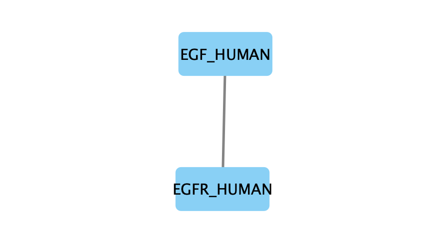
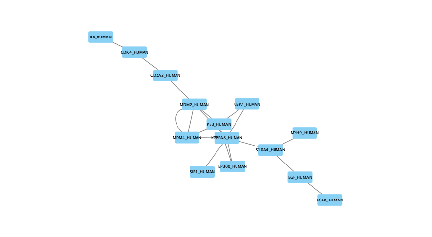
For example, the file egfr-pathlinker-params-7S4SLU6/pathway.txt contains the following reconstructed subnetwork:
Node1       Node2   Rank    Direction
EGF_HUMAN   EGFR_HUMAN      1       D
EGF_HUMAN   S10A4_HUMAN     2       D
S10A4_HUMAN MYH9_HUMAN      2       D
K7PPA8_HUMAN        MDM2_HUMAN      3       D
MDM2_HUMAN  P53_HUMAN       3       D
S10A4_HUMAN K7PPA8_HUMAN    3       D
K7PPA8_HUMAN        SIR1_HUMAN      4       D
MDM2_HUMAN  MDM4_HUMAN      5       D
MDM4_HUMAN  P53_HUMAN       5       D
CD2A2_HUMAN CDK4_HUMAN      6       D
CDK4_HUMAN  RB_HUMAN        6       D
MDM2_HUMAN  CD2A2_HUMAN     6       D
EP300_HUMAN P53_HUMAN       7       D
K7PPA8_HUMAN        EP300_HUMAN     7       D
K7PPA8_HUMAN        UBP7_HUMAN      8       D
UBP7_HUMAN  P53_HUMAN       8       D
K7PPA8_HUMAN        MDM4_HUMAN      9       D
MDM4_HUMAN  MDM2_HUMAN      9       D
The pathway.txt files serve as the foundation for further analysis, allowing you to explore and interpret the reconstructed networks in greater detail. In this case you can visulize them in cytoscape or compare their statistics to better understand these outputs.
4.2 Reviewing Outputs in Cytoscape and Summary Files
Open Cytoscape
Launch the Cytoscape application on your computer.
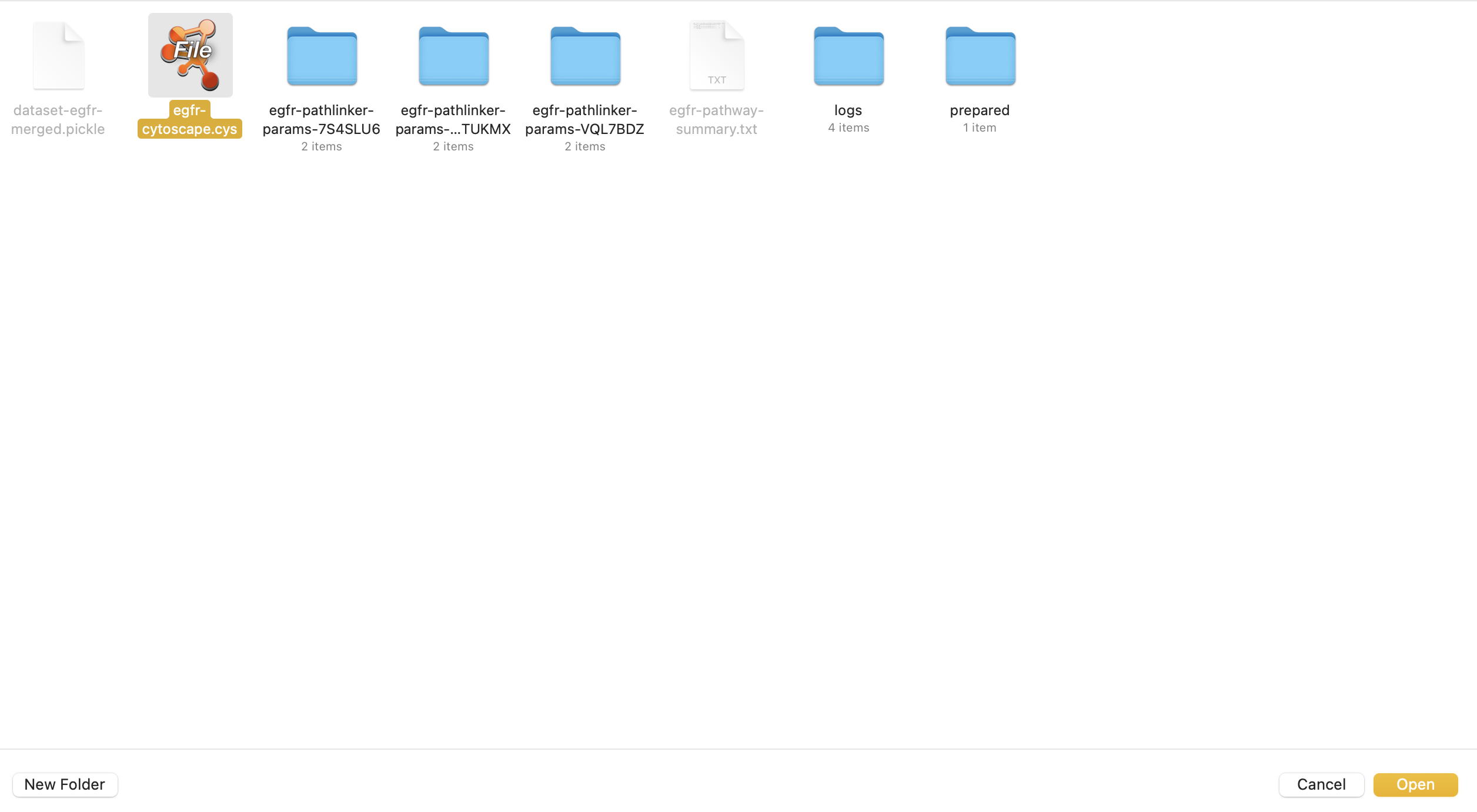
Load the Cytoscape session file
Navigate to spras/output/basic/egfr-cytoscape.cys and open it in Cytoscape.
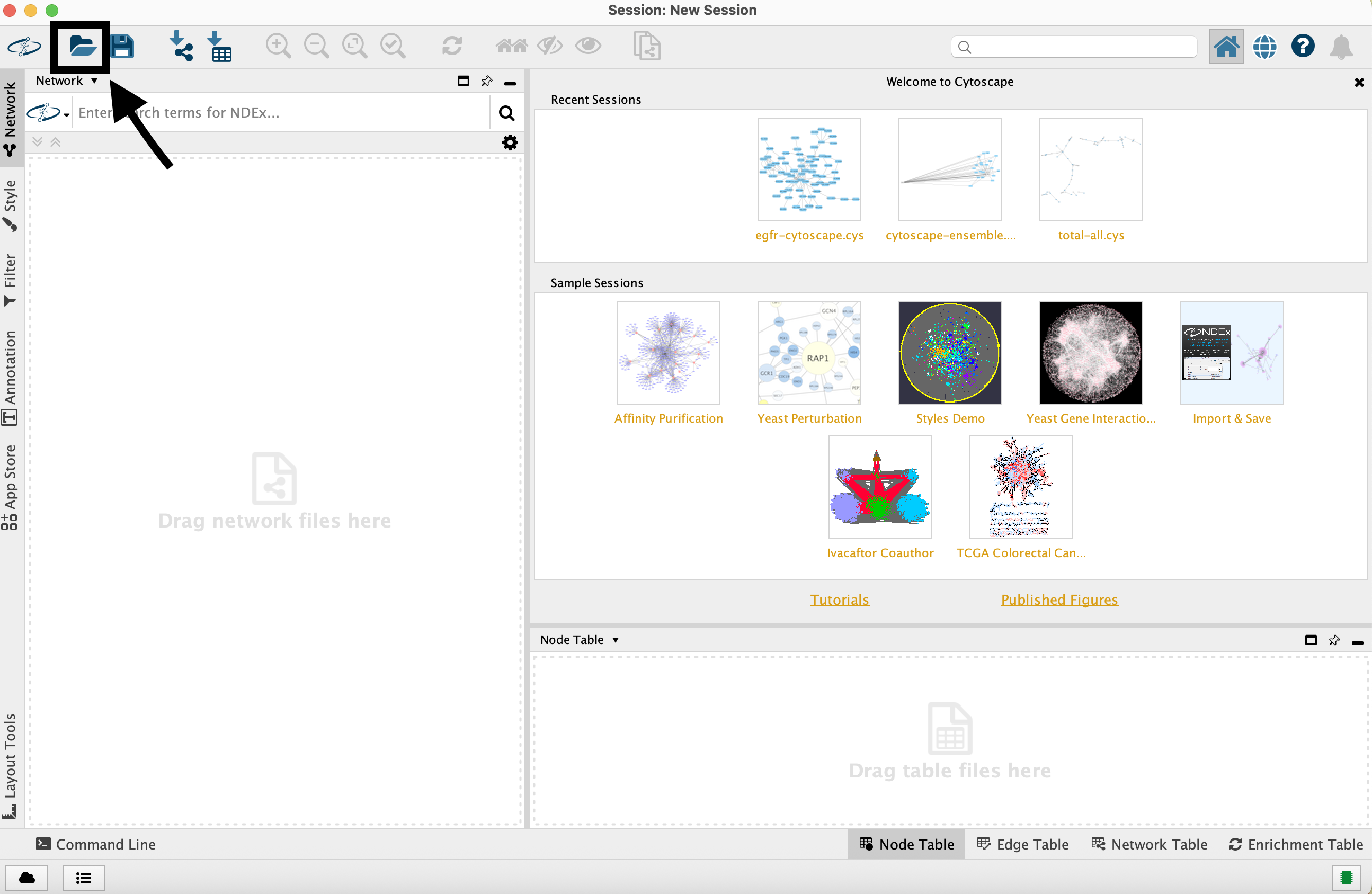
Once loaded, the session will display all reconstructed subnetworks for the chosen dataset, organized by algorithm and parameter combination.
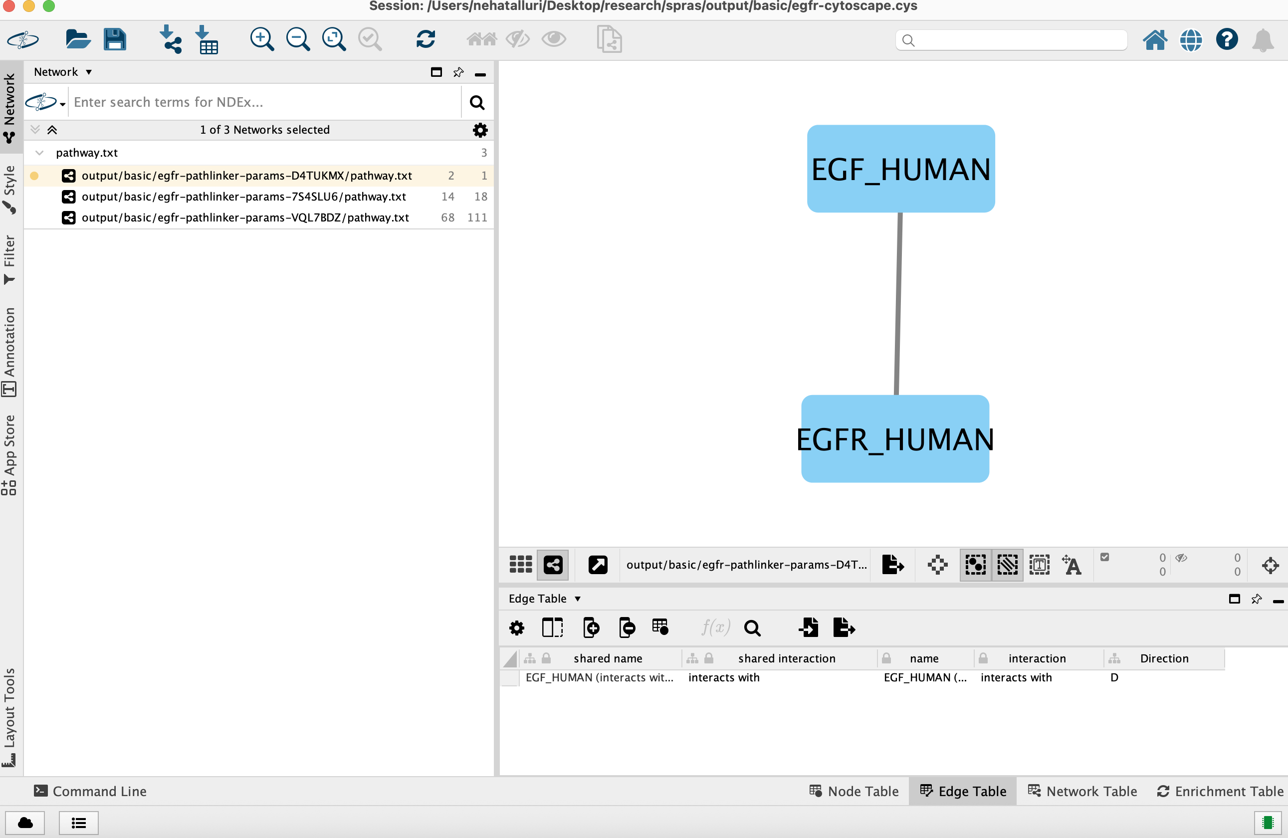
You can view and interact with each reconstructed subnetwork. Compare how the different parameter settings influence the pathways generated.
Open the summary statistics file
In your file explorer, go to spras/output/basic/egfr-pathway-summary.txt and open it locally.
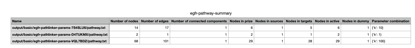
This file contains calculated statistics (e.g., number of nodes, edges, density, connected components) for each pathway.txt file, along with the parameter combinations that produced them.
By reviewing this file, you can interpret and compare algorithm outputs side by side using their statistics.
4.3 Comparing Across Parameter Combinations
As you compare across parameter settings, notice how the reconstructed subnetworks change based on the different parameters used:
The small parameter value (k=1) produced a compact subnetwork that highlights only the top-ranked interactions.
The moderate parameter value (k=10) expanded the subnetwork, introducing additional nodes and edges that may uncover new connections but increase complexity.
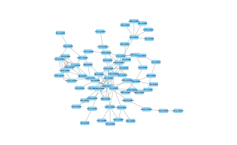
The large parameter value (k=100) generates a much denser subnetwork, capturing a broader range of edges but also could introduce connections that may be less meaningful.
Because the parameters used help determine which edges and nodes are included, each setting produces a different subnetwork. By examining the statistics (egfr-pathway-summary.txt) alongside the visualizations (Cytoscape), you can assess how parameter choices influence both the structure and interpretability of the outputs.